pseudospectral-method

1 伪谱法应用于最优控制问题

伪谱法 (Pseudospectral Method) 利用正交多项式根作为非均匀离散配点, 通过插值多项式对系统的状态与控制变量进行参数化处理. 相较于传统配点法, 伪谱法能够利用较少的离散节点实现更高的近似精度,避免了传统均匀插值方法产生的“龙格”现象,具有对初值不敏感, 收敛性良好的优点, 适用性广, 具备在线轨迹规划应用的潜力. 依据积分方法与离散节点配置的不同, 可以将伪谱法分为 Legendre-Gauss(LG) 伪谱法,Legendre-Guass-Lobatto(LGL) 伪谱法,Chebyshev-Guass-Lobatto(CGL) 伪谱法,Legendre-Guass-Radau(LGR)伪谱法等方法.

1.1 最优控制分类

动力下降问题分类1^[1-3]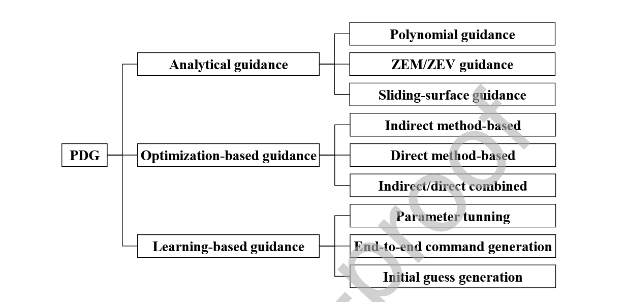

图 1: PDG 分类

动力下降问题分类2^[4]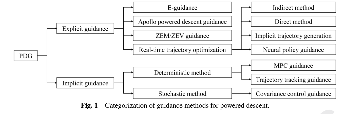

图 2: PDG 分类

数值方法分类^[5-6] 直接法分类

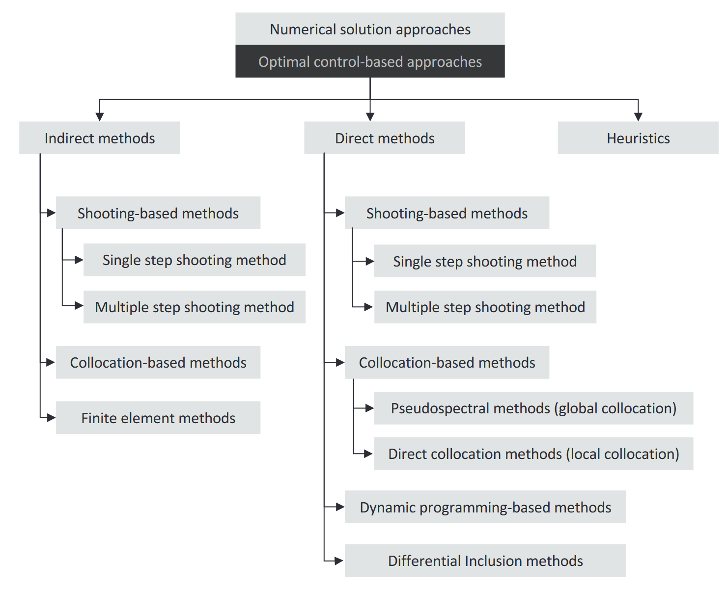
图 3: Numerical solution approaches

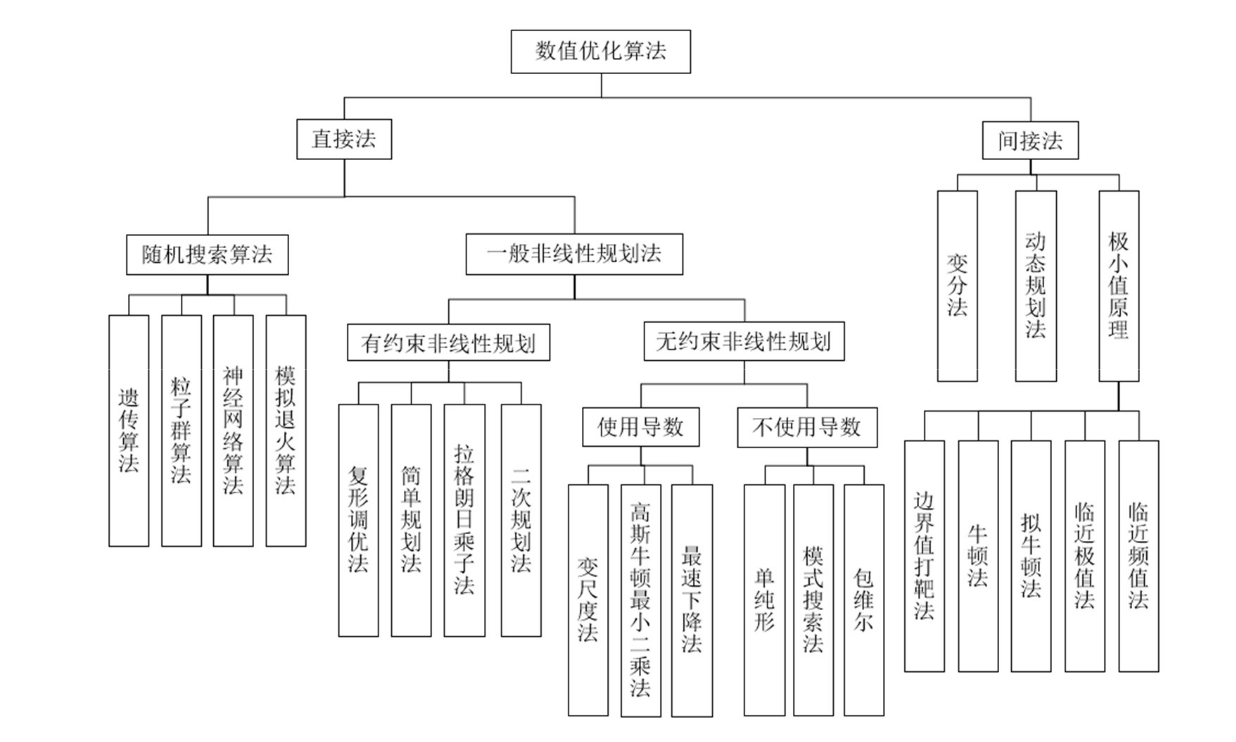
图 4: Numerical solution approaches

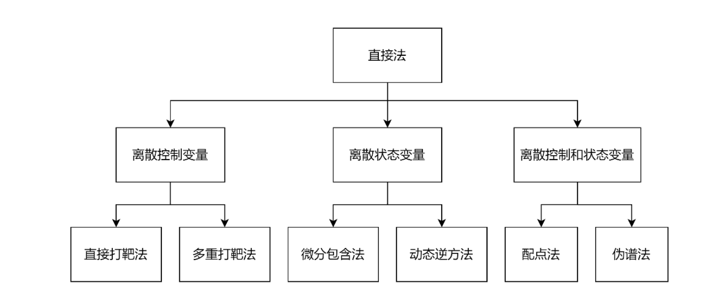
图 5: Numerical solution approaches

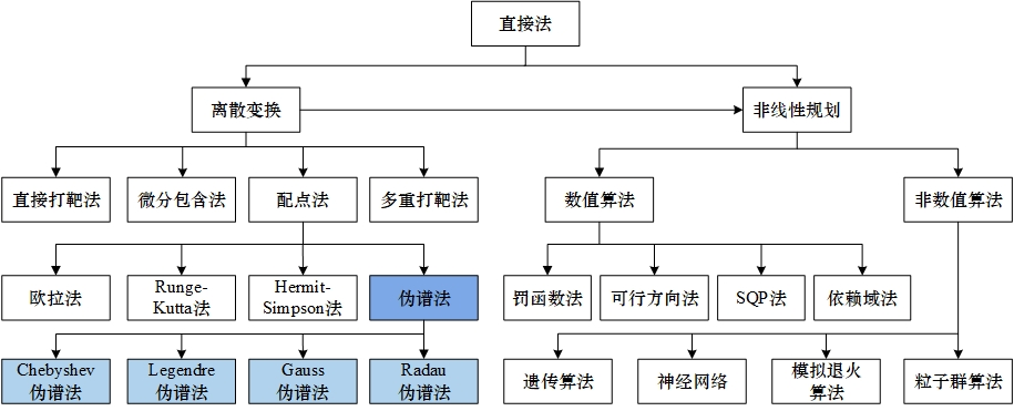
图 6: Numerical solution approaches

1.2 使用 LGR 配点的 RPM 方法

LPM 和 GPM 作为直接法都能将最优控制问题通过在配点处离散转化为 NLP, 具备指数收敛速度, 但是 LPM 配点在两个边界处的特点使得其对协态的估计并不准确.GPM没有这个问题, 能够证明使用 GPM 的 NLP 与原连续时间最优控制问题具有等价性, 然而, 在初始边界处的控制并不是从 NLP 解中获得的. 相比之下,RPM 下的 NLP 最优性条件与原问题等价, 同时能直接解出初始控制量,并且复杂度明显低于 RPM^[7].

1.2.1 拉格朗日多项式 (Lagrange polynomials)

在N+1 个节点上的N 次拉格朗日插值多项式有如下表述^[8]: $$ L_{i}(\tau) = \prod_{\substack{j = 1\\ j\neq i}}^{N}\frac{\tau - \tau_{j}}{\tau_{i} - \tau_{j}},\quad (i = 0,\ldots ,N). $$ 若引入记号 g_N(τ) = (τ − τ₀)(τ − τ₁)…(τ − τ_n),  n = 0, 1, 2, …. 易得 g_N^′(τ_k) = (τ_k − τ₀)…(τ_k − τ_k − 1)(τ_k − τ_k + 1)…(τ_k − τ_n),  n = 0, 1, 2, …. 故拉格朗日插值基函数可写为： $$ L _ {j} (\tau) = \frac {g _ {N} (\tau)}{g _ {N} ^ {\prime} (\tau_ {j}) (\tau - \tau_ {j})}, \quad g _ {N} (\tau) = \prod_ {j = 0} ^ {N} (\tau - \tau_ {j}). $$ 利用拉格朗日多项式近似的函数可以表示如下: $$ u (x) = \sum_ {j = 0} ^ {n} u _ {i} l _ {i} (x)\tag{1} $$ 则u的一阶导数可以表述如下: $$ u ^ {\prime} (x) = \sum_ {j = 0} ^ {n} u _ {i} l _ {i} ^ {\prime} (x)\tag{2} $$ 微分矩阵可由如下式推出(其中i=j处的微分矩阵元素值可由洛必达法则求极限得到)^[9]: $$ D _ {i j} = \left\{ \begin{array}{l l} \frac {g _ {N} ^ {\prime} (t _ {i})}{g _ {N} ^ {\prime} (t _ {j})} \frac {1}{t _ {i} - t _ {j}}, & i \neq j, \\ \frac {g _ {N} ^ {\prime \prime} (t _ {i})}{2 g _ {N} ^ {\prime} (t _ {i})}, & i = j. \end{array} \right. $$ 利用重心拉格朗日插值^[10]可以将微分项简化为 $$ \begin{array}{r l} & l _ {j} ^ {\prime} (x _ {i}) = \frac {w _ {j} / w _ {i}}{x _ {i} - x _ {j}} \\ & l _ {j} ^ {\prime} (x _ {j}) = - \sum_ {i \neq j} l _ {j} ^ {\prime} (x _ {i}) \end{array}\tag{3} $$

其中 $$ w _ {j} = \frac {1}{\prod_ {k \neq j} (x _ {j} - x _ {k})}, \quad j = 0, \dots , n\tag{4} $$

1.2.2 勒让德多项式 (Legendre polynomial)

1814年罗德利克 (Rodrigul)给出了勒让德多项式的简单表达式^[11] $$ P _ {N} (\tau) = \frac {1}{2 ^ {N} N !} \frac {d ^ {N}}{d \tau^ {N}} \big [ (\tau^ {2} - 1) ^ {N} \big ] $$ 勒让德多项式根难以直接计算，一般采用如下递推方法结合牛顿法求解: $$ \begin{array}{c} P _ {0} (t) = 1 \\ P _ {1} (t) = t \\ (N + 1) \cdot P _ {N + 1} (t) = (2 N + 1) \cdot t \cdot P _ {N} (t) - N \cdot P _ {N - 1} (t), \quad N \geq 1 \end{array} $$ 勒让德多项式还有以下恒等式(wiki上的,书本还没找到): $$ \begin{array}{c} \frac {x ^ {2} - 1}{n} \frac {d}{d x} P _ {n} (x) = x P _ {n} (x) - P _ {n - 1} (x) \\ \frac {d}{d x} P _ {n + 1} (x) = (n + 1) P _ {n} (x) + x \frac {d}{d x} P _ {n} (x) \\ (2 n + 1) P _ {n} (x) = \frac {d}{d x} (P _ {n + 1} (x) - P _ {n - 1} (x)) \end{array}\tag{5} $$

1.2.3 Legendre-Gauss-Radau(LGR) 伪谱法

LGR 伪谱法即 RPM 作为一种直接法, 已经经历了十足的探索^{[12-13,9,7,14-18]}, 其采用LGR配点作为原连续最优控制问题的非均匀离散点,使得原问题转换为可以求解的有限维非线性规划问题.LGR配点是如下 N 阶 LGR多项式在区间[ 1,1) 上的根: R_N = P_N − 1(τ) + P_N(τ) 其中 P_N 和 P_N 分别为 N 阶以及 N-1 阶勒让德多项式. 利用勒让德多项式的递推公式与牛顿法可以解得原方程的数值解. 考虑 N 个 LGR 配点, (τ₁, τ₂, …, τ_n) , 其中 τ₁ = −1 并且 τ_N < +1 . 新增右端点 τ_N + 1 = 1 作为节点. 注意到该节点并不属于 LGR 配点^[13], 但是增加该节点有助于表述末端状态量. 因此对于一般 LGR 方法或 f-LGR 方法, 初始控制量/末端控制量需要在求解完 NLP 问题后外推得到^[19,17]. 由于所有伪谱法的归一化时间间隔为 τ ∈ [−1, 1] ], 原最优控制问题的时间跨度为 t ∈ [t₀, t_f] , 因此存在如下时域变换关系: $$ \begin{array}{l l} & t = \frac {t _ {f} - t _ {0}}{2} \tau + \frac {t _ {f} + t _ {0}}{2} \\ t \in [ t _ {0}, t _ {f} ] & \xleftarrow {} \quad \tau \in [ - 1, 1 ] \end{array} $$ 在这种方法下, 原动力学方程可以表示如下: $$ \dot {x} (\tau) = \frac {t _ {f} - t _ {0}}{2} f (x (\tau), u (\tau), \tau)\tag{7} $$

$$ \begin{array}{c} \dot {x} (\tau) \approx \dot {X} ^ {N} (\tau) = \sum_ {k = 1} ^ {N + 1} X _ {i} \dot {L} _ {i} (\tau) = \sum_ {k = 1} ^ {N + 1} D _ {i k} x (\tau_ {k}) \\ \sum_ {k = 1} ^ {N + 1} D _ {i k} x (\tau_ {k}) = \frac {t _ {f} - t _ {0}}{2} f (x (\tau_ {i}), u (\tau_ {i}), \tau_ {i}), \quad i = 1, \dots , N. \end{array}\tag{8} $$ 对于包含右侧端点的最优控制问题,微分矩阵 D = [D_ik] 并不是方阵. 最后,对于一般控制问题的 Bolza型代价函数: $$ J = \Phi (y (- 1), t _ {0}, y (+ 1), t _ {f}) + \frac {t _ {f} - t _ {0}}{2} \int_ {- 1} ^ {1} g (y (\tau), u (\tau), \tau ; t _ {0}, t _ {f}) d \tau\tag{9} $$ 利用 LGR 求积近似为: $$ J = \Phi \big (Y (\tau_ {1}), \tau_ {1}, Y (\tau_ {N + 1}), \tau_ {N + 1} \big) + \frac {t _ {f} - t _ {0}}{2} \sum_ {k = 1} ^ {N} w _ {k} g \big (Y _ {k}, U _ {k}, \tau ; t _ {0}, t _ {f} \big)\tag{10} $$ LGR求积公式有下面两种表述^[8]: $$ w _ {i} = \left\{ \begin{array}{l} \frac {2}{N ^ {2}}, \quad i = 1, \\ \frac {1}{(1 - \tau_ {i}) \big [ \dot {P} _ {N - 1} (\tau_ {i}) \big ] ^ {2}} = \frac {1 - \tau_ {i}}{[ N \cdot P _ {N - 1} (\tau_ {i}) ] ^ {2}}, \quad 2 \leq i \leq N. \end{array} \right. $$

1.2.4 仅包含单侧端点

参考文献

[1] WANG J, ZHANG R, LI H. Disturbance rejection and convex optimization-based guidance for autonomous shipborne landing of a reusable rocket[J]. Aerospace Science and Technology, 2026: 111917.

[2] SONG Z Y, WANG C, THEIL S, et al. Survey of autonomous guidance methods for powered planetary landing[J]. Frontiers of Information Technology & Electronic Engineering, 2020, 21(5): 652-674.

[3] 张晓文, 王天舒, 王大轶, 等. 行星动力下降多约束最优反馈制导方法[J]. 宇航学报,2023, 44(8): 1171-1182.

[4] CHEN X, ZHANG R, LI H. Optimal feedback guidance with disturbance rejection for endoatmospheric powered descent[J]. Chinese Journal of Aeronautics, 2024: 103336.

[5] CHAI R, SAVVARIS A, TSOURDOS A, et al. A review of optimization techniques in spacecraft flight trajectory design[J]. Progress in Aerospace Sciences, 2019, 109: 100543.

[6] 杨智超. 可回收火箭动力下降轨迹优化及制导方法研究[D]. 哈尔滨工程大学, 2025.

[7] GARG D, PATTERSON M A, FRANCOLIN C, et al. Direct trajectory optimization and costate estimation of finite-horizon and infinite-horizon optimal control problems using a radau pseudospectral method[J]. Computational Optimization and Applications, 2011, 49 (2): 335-358.

[8] ABRAMOWITZ M E, STEGUN I A E. Handbook of mathematical functions with formulas, graphs, and mathematical tables[M]. U.S. Department of Commerce, National Bureau of Standards, 1964.

[9] FAHROO F, ROSS I M. Advances in pseudospectral methods for optimal control[C]// AIAA Guidance, Navigation and Control Conference and Exhibit. Honolulu, Hawaii: American Institute of Aeronautics and Astronautics, 2008.

[10] BERRUT J P, TREFETHEN L N. Barycentric lagrange interpolation[J]. SIAM Review, 2004, 46(3): 501-517.

[11] 李庆阳. 数值分析: 第 6 版[M]. 北京: 清华大学出版社, 2025.

[12] GARG D, PATTERSON M, HAGER W W, et al. A unified framework for the numerical solution of optimal control problems using pseudospectral methods[J]. Automatica, 2010, 46(11): 1843-1851.

[13] GARG D. Advances in global pseudospectral methods for optimal control[D]. USA: University of Florida, 2011.

[14] TANG X, CHEN J. Direct trajectory optimization and costate estimation of infinitehorizon optimal control problems using collocation at the flipped legendre-gauss-radau points[J]. IEEE/CAA Journal of Automatica Sinica, 2016, 3(2): 174-183.

[15] XIE L, ZHANG H, ZHOU X, et al. Hp-adaptive Pseudospectral Convex optimization for Rocket Powered Landing Trajectory Planning[C]//2019 Chinese Automation Congress (CAC). 2019: 895-900.

[16] ZHANG T, SU H, GONG C. Hp-adaptive RPD based sequential convex programming for reentry trajectory optimization[J]. Aerospace Science and Technology, 2022, 130: 107887.

[17] SAGLIANO M. Pseudospectral convex optimization for powered descent and landing[J]. Journal of Guidance, Control, and Dynamics, 2018, 41(2): 320-334.

[18] CANNATARO B Ş, RAO A V, DAVIS T A. State-defect constraint pairing graph coarsening method for karush–kuhn–tucker matrices arising in orthogonal collocation methods

for optimal control[J]. Computational Optimization and Applications, 2016, 64(3): 793- 819.

[19] SAGLIANO M, THEIL S, BERGSMA M, et al. On the radau pseudospectral method: Theoretical and implementation advances[J]. CEAS Space Journal, 2017, 9(3): 313-331.